How Does Machine Learning Work?
Before an AI is ready for use, it must be trained for the task at hand. In the following, we go step by step through the individual phases of machine learning.
Required Imports
import torch
import torch.utils as utils
import torchvision
from torchvision import datasets, transforms
import matplotlib.pyplot as plt

# check torch install
print(torch.__version__)
Basic Definitions
# Path to dataset
dataset_path = "Dataset"

# numberand names of classes
num_classes = 4
classes = ("glass", "metal","paper","plastic")
Transformations
PyTorch transformations are crucial because they facilitate data preprocessing, augmentation, and preparation, which are essential for training robust and accurate machine learning models. Here are some important transformations:
- Normalization: Transformations allow normalization of data to standardize input features. For example, image pixel values can be scaled to a specific range (e.g., 0–1 or -1–1) to make training more stable.
- Tensor Conversion: Converting raw data (e.g., images or arrays) to PyTorch tensors is necessary for compatibility with PyTorch models.
- Resizing: Standardizing the input size for a consistent model input.
- Cropping: Focusing on specific regions of an image.
- Flipping/Rotating: Creating variations to improve model generalization.
transformations = transforms.Compose([
        transforms.Resize(224),
        transforms.RandomVerticalFlip(),
        transforms.RandomHorizontalFlip(),
        transforms.RandomResizedCrop(224),
        transforms.ToTensor(),
        transforms.Normalize([0.485, 0.456, 0.406], [0.229, 0.224, 0.225])
    ])


dataset = datasets.ImageFolder(dataset_path, transform = transformations)
classes = dataset.classes
Deviding the Dataset
The next step is to divide the entire data set into training data and test data. A division of approx. 80% training data and 20% test data has proven to be successful.
train_subset , test_subset = utils.data.random_split(dataset, [2000,523],
        generator = torch.Generator().manual_seed(1))
train_subset.dataset.transform = transformations
Defining the Dataloaders
A PyTorch DataLoader is a utility in the PyTorch library that simplifies and automates the process of loading and managing data for machine learning models. It is particularly useful when working with large datasets that cannot fit into memory at once or when you need to apply data transformations and batching efficiently. We define a data loader for the training data and one for the test data:
train_loader = utils.data.DataLoader(train_subset, batch_size=4, shuffle=True, num_workers=0)
test_loader = utils.data.DataLoader(test_subset, batch_size=4, shuffle=True, num_workers=0)

dataloaders = {"train": train_loader, "test": test_loader}
Training Algorithm
Now comes the most important part: the program for training the neural network. The function has 3 parameters: the model, the data loaders used and the number of epochs that are run through in the training:
def training_and_test(model, dataloaders, epochs ):

    # lists for data evaluation
    train_acc =[]   # training accuracy
    test_acc = []   # test accuracy
Each epoch has two phases: a training phase in which the training data is learned and a test phase in which the network is tested against the test data:
    # phases
    phases = ["train", "test"]
Optimizer
In PyTorch, an optimizer is a key component of the machine learning workflow, responsible for adjusting the parameters (weights and biases) of a model during training in order to minimize the loss function. It implements specific optimization algorithms, such as Stochastic Gradient Descent (SGD), Adam, or RMSprop, among others. We use Adam.
    params_to_update = []  # list to store the names of the parameters that will be updated
    for name, param in model.named_parameters():
        if param.requires_grad:
            # Add the parameter to the list if requires_grad is True
            params_to_update.append(param)
            # Print the name of the parameter
            print("\t", name)
    optimizer = optim.Adam(params_to_update)
Loss Function
A PyTorch loss function is a key component in training machine learning models with the PyTorch library. Loss functions are mathematical formulations that measure the difference between the model's predictions and the true target values. By minimizing this loss during training, the model improves its performance.
In PyTorch, loss functions are implemented as classes or functions found in the torch.nn module or as standalone methods in the torch namespace. They are typically used in conjunction with optimization algorithms (e.g., torch.optim.SGD, torch.optim.Adam) to adjust the model's weights.
Cross-Entropy Loss
Cross-entropy loss, also known as log loss, is a widely used loss function in machine learning, particularly for classification tasks. It measures the difference between two probability distributions: the predicted probability distribution produced by the model and the true (target) distribution from the data. It is particularly well-suited for tasks involving multi-class classification.
errorfunction = torch.nn.CrossEntropyLoss()
Now let's start ...
    # go through the training loop for all epochs
    for epoch in range(epochs):
        print("Epoch ", epoch + 1, " of " , epochs )

        # carry out training and then evaluation phases
        for phase in phases:
            if phase == 'train':
                model.train()  # training mode
            else:
                model.eval()  # test mode

            # Number of correct predictions
            correct = 0

            # Iterate over all data
            for inputs, labels in dataloaders[phase]:

                # Reset the gradient of the optimizer after each run
                optimizer.zero_grad()

                # One pass (gradient calculation on or off)
                with torch.set_grad_enabled(phase == 'train'):
                    # Chasing input through the network and calculating output
                    outputs = model(inputs)

                    # Apply error function -> Calculate error
                    error = errorfunction(outputs, labels)

                    # The maximum value is the predicted class
                    _, predicted = torch.max(outputs, 1)

                    # Optimize model (only in training)
                    if phase == 'train':
                        # Using backpropagation
                        error.backward()
                        # Recalculate weights
                        optimizer.step()

                # Number of correctly determined labels
                correct = correct + torch.sum(predicted == labels.data)

            # Calculate the accuracy of the forecast
            accuracy = correct.double() / len(dataloaders[phase].dataset)

            print("accuracy in phase ", phase, " : ", accuracy)

            # Save current accuracy in our history
            if phase == 'test':
                test_acc.append(accuracy.item())
            else:
                train_acc.append(accuracy.item())
    # return the trained model and the test history as a result
    return  model, train_acc, test_acc
Selecting A Model
There are many different types of artificial neural networks. These include: Perceptron, Feed Forward Neural Networks, Convolutional Neural Networks and Recurrent Neural Networks. Convolutional neural networks (CNNs) are used in particular in the field of image processing. In the case of CNNs, there are several layers (similar to multi-layer feedforward networks) that follow one another. There are three types of layers here: Convolutional Layer, Pooling Layer and Fully-Connected Layer.
Recurrent Neural Networks
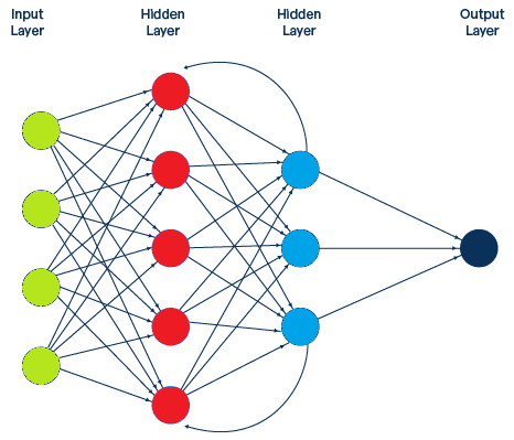
In contrast to feedforward networks, some artificial neurons in recurrent neural networks (RNNs) are fed back. Put simply, the output of an artificial neuron is fed back as input to the same or previously used neuron (so-called feedback loop). In this way, the RNNs can retain information within an artificial neuron. In this respect, the RNNs have a kind of memory.

For this tutorial I use ResNet18, of course you can also use other CNNs or Recurrent Neural Networks.
model = torchvision.models.resnet18(weights=torchvision.models.ResNet18_Weights.DEFAULT)
model.fc = torch.nn.Linear(model.fc.in_features, 4)

model , train_hist, test_hist = training_and_test(model, {"train" : train_loader, "test" : test_loader}, 20)
Saving the Trained Model
After the training i save the models so that i can use them again later for my application:
datestring = datetime.now().strftime("%m_%d_%Y_%H_%M_%S")
torch.save(model.state_dict(), "model_" + datestring + ".pth")
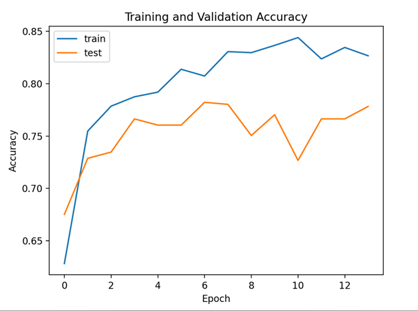
Visualize Training Progress
plt.plot(train_hist,label="train")
plt.plot(test_hist,label="test")
plt.legend()
plt.show()
