Training Process
Selecting a Model
The choice of a neural network depends very much on the task and requires experience. Fortunately, the digit dataset is so easy to learn that even a very simple neural network can do it without any problems.
We can use the “MLPClassifier” network from SCIKIT-LEARN for this. The network automatically adapts the input layer to the problem size, in our case it also consists of 8 x 8 = 64 neurons. The output layer results from the number of objects to be classified, for the digits from 0 to 9 we need 10 neurons in the output layer.
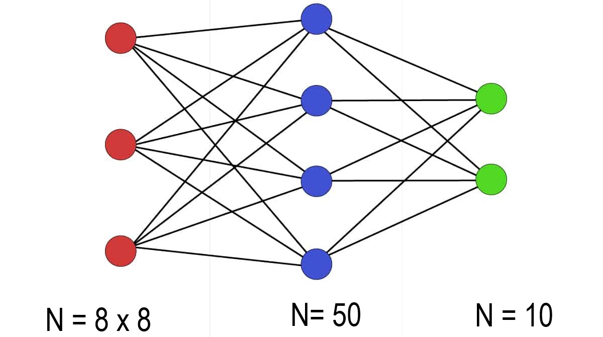
The following program generates a simple feed-forward network with 50 neurons in the hidden layer and outputs the most important parameters of the network.
from sklearn.neural_network import MLPClassifier

model = MLPClassifier(hidden_layer_sizes=(50,), max_iter=500)
params = model.get_params()
for key, value in params.items():
    print(key + " : " + str(value))
Preparing the Dataset
The division into training and test data is a central component of machine learning. Here is a brief explanation with reasons:
Training data: This data is used by the model to learn patterns - i.e. the “learning phase”.Test data: This data is used after the model has been trained to evaluate performance - without the model having seen this data beforehand.
Why is this important? To avoid overfitting: If you train the model on all available data, it could "memorize" the data instead of learning real patterns. This is called overfitting. It would then be good on the training data, but bad on new data.
Objective evaluation of model performance: Test data is the only way to really assess how well the model works on unknown data - i.e. in reality.
The usual split is 70 to 80% training and 20 to 30% test data. We use a 30 / 70 split here. The following program splits the data and the labels 70 to 30 and outputs the number of the respective images and labels
from sklearn import datasets
from sklearn.model_selection import train_test_split

# Datensatz laden
digits = datasets.load_digits()


# 70% sind Trainingsdaten, 30% sind Testdaten
bilder_train, bilder_test, labels_train, labels_test = train_test_split(
    digits.data, digits.target, test_size=0.3, random_state=42)

print("Bilder für das Training: " , len(bilder_train) )
print(bilder_train)
print("Labels für das Training: " , len(labels_train))
print(labels_train)
print("Bilder für den Test:  " , len(bilder_test) )
print(bilder_train)
print("Labels für den Test:" , len(labels_test))
print(labels_train)
Training
the training is as simple as possible: you set the number of maximum epochs in the model,
call up the “fit” method and transfer the training data and labels. The parameter “verbose”
provides an output of the training progress.
There is also a very simple “score” method for the evaluation.
from sklearn.neural_network import MLPClassifier
from sklearn import datasets
from sklearn.model_selection import train_test_split
import joblib

# Datensatz laden
digits = datasets.load_digits()

# 70% sind Trainingsdaten, 30% sind Testdaten
bilder_train, bilder_test, labels_train, labels_test = train_test_split(
    digits.data, digits.target, test_size=0.3, random_state=42)

# Modell erzeugen: 50 neuronen in der hidden layer
model = MLPClassifier(hidden_layer_sizes=(50,), max_iter=500, verbose = True)

# Training
model.fit(bilder_train, labels_train)

# Auswertung
print("Genauigkeit mit Trainingsdaten nach Training:", model.score(bilder_train, labels_train))
print("Genauigkeit mit Testdaten nach Training:", model.score(bilder_test, labels_test))

# Modell speichern
joblib.dump(model, 'digits_model.pkl')
The program for the traininig then provides the following output:
.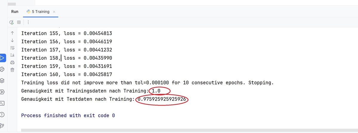
you can see that the optimizer has aborted the training process after 168 iterations because
there has been no further improvement in accuracy in the last 10 epochs.
If you look at the accuracy achieved, you can see that 100% was achieved for the training data and 97% for the test data.